This article aims to present a possible use of Lekan, version 2.3, with a concrete case of constructing a 2D hydraulic model of a river, from the preparation of topographic data to the visualization of results.

At the end of this article, new possibilities that are opened up with ongoing work are also presented (only for the experimental version), through the possibility of interacting with a project via a Python API. The use case is then to automate the resolution of the previous model to produce real-time flood field raster data.

 

The choice of the study area was made in order to gather data that can be currently used without requiring additional acquisition. It is evident that not all areas can have usable data as in this use case. This biased choice is deliberate for demonstration purposes. Applying this use case to other areas may require acquiring additional data.

The chosen area corresponds to a section of a river in a particular sector:

• Included in the current coverage of IGN’s HD LIDAR data
• With relatively low vegetation cover, allowing for a suitable digital terrain model to be obtained from LIDAR data.
• With a hydrometric station providing “real-time” flow rates from the Hub’Eau service.

The IGN has started providing high-definition LIDAR surveys in the form of point clouds, allowing for extremely precise restitution of terrestrial topography. However, the data currently provided is raw and unclassified. This results in a set of points containing both natural terrain and vegetation, buildings, and any existing structures. While these data can constitute a digital surface model (DSM), the crucial data for any hydraulic model is the digital terrain model (DTM), which includes only the surfaces of the terrain without vegetation and structures that are more or less transparent to flow.

With a classified LIDAR survey, meaning that each point is associated with a type (terrain, vegetation, building, etc.), it is easy to obtain a DTM after filtering out these categories.

Unfortunately, the IGN’s LIDAR survey is currently not classified. This requires a more complex processing. For this processing, the free and open-source software Cloud Compare offers some algorithms to sort the data. This is convenient because Cloud Compare also allows the creation of a raster DTM from point clouds.

Once the raster DTM is exported to GeoTIFF format, a small clean-up in QGIS is necessary to remove the triangulations on the edges and impose the coordinate system.

Since the use of Cloud Compare and QGIS is not the subject of this article, we will not dwell on this processing, and we will simply show the before/after.

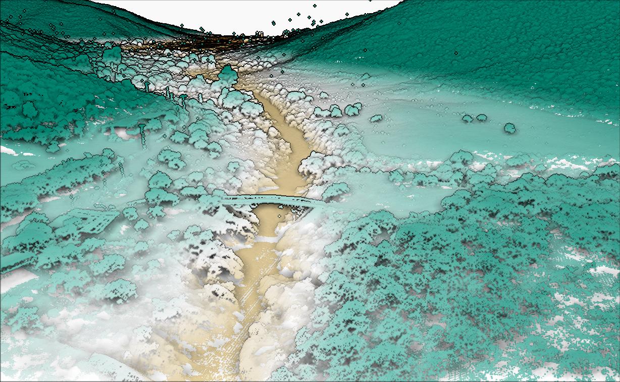
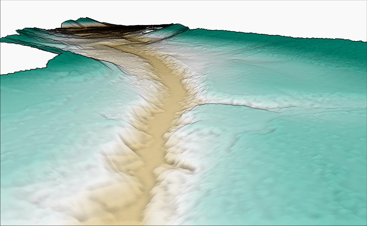
Limitation of the méthod

The processing carried out here is global and can lead to inaccuracies and errors in the DTM. Indeed, the filtering process removes a significant number of points based on certain criteria, and some points of the natural terrain can be removed, resulting in “holes” in the point cloud. The conversion to a raster format then interpolates elevation values in these holes based on the surrounding points, usually by triangulation. These interpolations are then clearly visible in the raster DTM and, depending on their importance, can influence the modeling results.

Now that we have a DTM with more than adequate precision, despite some questionable interpolations, we can import it into Lekan.

Geometry

The first step in building a 2D model is entering the domain of the model.

When the user adds a 2D structure (name of 2D model under Lekan), the domain is directly entered on the map.

It is also possible to use a polygon from an existing vector layer, selected by right-clicking on the polygon during domain entry.

Once the domain entry is complete, entering the editing window, via the properties window of this new element of the hydraulic network, allows for model editing.

 

The editing window of the 2D structure allows for all model construction operations to be performed from several pages, each dedicated to:

• Editing the general structure
• Adjusting mesh resolution
• Topography to apply on the mesh
• Editing individual or group faces and vertices and verifying mesh quality
• Model roughness by zone
• Adjusting simulation settings
• Definition of the time window, i.e. the start and end dates and times of the simulation.

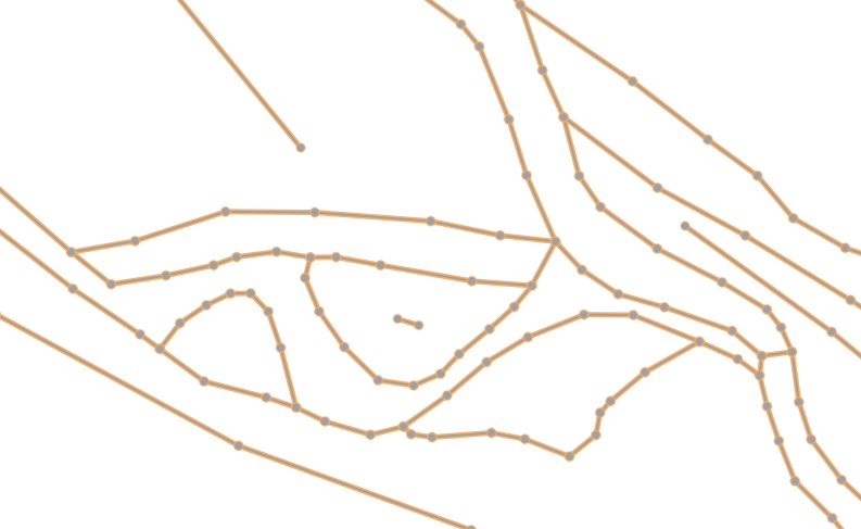
From the “Structure” page, the user can edit the structure lines of the model, i.e. the domain as well as internal structure lines, add holes in the domain, and insert boundary conditions.

It is also here where the choice of the algorithm for mesh generation is made. Lekan uses the Gmsh generator internally. This generator offers different algorithms for mesh generation. We will use the BAMG algorithm here, which allows for a very regular triangulation.

Clicking on “Generate mesh” will start the mesh generation with the default resolution.

 

Even though this mesh could benefit from further refinement through structure lines, it is now possible to apply a topography for an initial visualization. This is done on the “Topography” page. Here, the user adds one or more DTM to a list that will be used to apply an elevation value to each mesh vertex.

The overlay of multiple DTMs in a list allows for combining several DTMs: if the first DTM does not have a valid value at a vertex, the second DTM is used; if it does not have a valid value, the third one is used, and so on.

In our case, we use the DTM derived from HD LIDAR, and a much coarser DTM (25m resolution) for the few vertices on the periphery that are not covered by the fine DTM.

The “Apply Topography” button starts the process and allows for adding relief to our mesh. The “Terrain Styling” button can be used to customize the 2D rendering of the terrain elevation.

The 3D view is then very useful for controlling the quality of the mesh.

As expected, the mesh resolution does not seem sufficient, especially in the riverbed of our watercourse. It is therefore time to refine all of this.

 

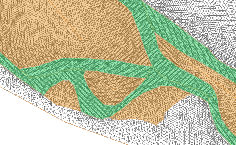
Adding structure lines allows drawing the outline of the riverbed and its bifurcations. The mesh resolution is defined by resolution classes associated with polygons drawn on the map. Right-clicking allows drawing a polygon defined by structure lines directly.

The “Edit elements / MeshQuality” page identifies elements (faces and vertices) that exceed certain quality thresholds. The user can then edit the elements individually to correct whatever they deem necessary based on his criteria. In our case, we will not change anything and move on to roughness.

Roughness

The roughness is defined in the same way as the mesh resolution, by polygons associated with value classes.

Here we arbitrarily create two value classes at 0.035 and 0.05 (Manning coefficient) for the main bed and middle bed, and give a default value of 0.1 to be applied everywhere else.

A right-click inside a polygon formed by structure lines allows to directly associate this polygon with a roughness class.

Note that the roughness values are completely arbitrary and, in a real study case, should be set more seriously. In our example, they should still allow us to obtain results.

 

Boundary condition

Entering the boundary conditions is done on the “Structure” page of the model editing by simply selecting the two vertices of the domain boundary defining the boundary conditions.

As the 2D structure is part of a hydraulic network that is connected to other elements through its boundary conditions, the type of boundary conditions depends on what it is connected to. Three cases are possible:

• Nothing is connected: the type of boundary conditions must be defined in its properties by the user.
• A link of the network arrives at it: the boundary condition is a flow inlet.
• A link of the network leaves it: the boundary condition is a water level condition.

In our case, we will use the flow rate from the Hub’Eau service. In Lekan, this flow rate will be produced in a node that we will connect to the upstream boundary condition.

For the downstream boundary condition, we will arbitrarily set a reasonable constant water level.

Station of the Hub’Eau service

The study area was partially chosen to be immediately downstream of a functioning hydrometric station present in the remote Hub-Eau database. It would therefore be a shame not to use it in our model.

To create a node directly corresponding to this station, you need to go through “Add a node from…”, select the source “Hub-Eau”, choose the correct station on the map, and add it.

To send its flow into the structure, simply create a link from the station node to the downstream boundary condition.

Tips :

The solver we are going to use is TELEMAC 2D with the “finite volume” equations. With this scheme, when the flow is torrential, the input flow condition in the model must be accompanied by information about the velocity profile. However, the section of the river here has a slope of around 1%, which will certainly result in torrential flow. Moreover, we will start the model “dry”, so the upstream section will certainly be in supercritical regime from the start.

Setting up the simulation

A simulation of a model corresponds to a solver and its intrinsic parameters. Here, we are dealing with a TELEMAC 2D simulation for which we need to specify:

• The time step of the simulation
• The initial conditions
• The numerical scheme (finite elements or finite volumes) and any associated parameters.

For the definition of initial conditions, there are several options:

• Fix a constant water level with zero velocity over the entire domain
• Use the result of another simulation of the same model
• Define the water level with zero velocity based on an interpolation line over the entire domain.

We will use this last solution here. Even though almost the entire model is “dry” at startup, we want the upstream section to be “wet” at startup at the location of the artificial depression. On the other hand, downstream, it is recommended to start with a level equal to the constant level we have set. Given the slope, the upstream level is about 10 m above the downstream level. Therefore, we cannot use a constant level over the entire model.

The principle of the interpolation line is explained here. By placing this interpolation line in a judicious manner and setting the value of the downstream water level on one side and a water level that allows “filling without overflowing” the artificial depression on the other side, we will have our desired initial conditions upstream and downstream.

Time window

The time window corresponds to the start and end dates/times. It can be defined either automatically based on the boundary conditions or directly by the user.

In our case, the hydrograph from the Hub’Eau server indicates the occurrence of a peak on April 15, 2023. We will simulate this peak by appropriately defining the manual time window.

At this point, the model construction is complete. All that remains is the simulation, which will only take a few minutes.

Once the simulation is complete, the user can visualize the flood field with:

1. plan view with values of water level, water height, flow velocity or terrain elevation using color palettes, visualization of vector velocity field with arrows, streamlines or traces (static or dynamic)
2. Longitudinal or cross-sectional profiles with terrain elevation, water level, and flow velocity
3. 3D view with mapping of water level, water height or flow velocity values

Below is a sample of result visualization from screenshots taken from Lekan (click to enlarge).

Currently under experimentation, an API for the Python language is being developed. This will make it possible to create and configure all elements of Lekan using Python code, as well as control them and exploit the results.

For example, if we take the model from this article, we can create a Python script that launches a simulation every time a new flow rate value is available on the upstream station’s. At the end of each simulation, the results are saved in raster format and can be sent, for example, to a database (which can be displayed on the web). The water level value is monitored at a specific point and an alert can be sent somewhere if it exceeds a certain threshold.

This 150-line script below thus constitutes a minimalist flood monitoring system and can be executed outside of Lekan.